DOURNAC.ORG
Français  English
Home
Astronomy
Sciences
Philosophy
Coding
Cv

Sciences > Correction of Probability Examination - Subatomic Physics Master's degree


  • 1.Gauss's law and Characteristic function
  • 2.Transfer Theorem
  • 3.Expectation and Statistical Variance in general case
  • 4.Making two no-correlated random variables
  • 5.Independance and no-Correlation of two random variables
  • 6.Maximum likelihood - 2 measure samples
  • 7.Maximum likelihood - 2 estimations with error
  • 8.Monte-Carlo method
  • 9.Generator of uniform law
  • 10.Chi2 method
  • 11.Chi2 method with measure errors
  • 12.Confidence level

Exercise 1.1 :

We consider a random variable $x$ on $]-\infty ,+\infty [$ following a Gauss’s law with $\mu $ and $\sigma $ parameters.

- Give the expression of Gauss’s law.
- Give the conditions on parameters to make this law be a probability distribution function (pdf).
- What is the Characteristic function (definition and expression) ?
- Do the same for cumulative function.

Reminder :

\begin{equation} \text{erf}(z)=\dfrac{2}{\sqrt{\pi}}\,{\large\int}_{0}^{z}\,exp(-t^{2})dt \end{equation}

Correction :

Let $x$ be a random variable defined on $]-\infty ,+\infty [$ and following a Normal distribution (Gaussian).

Distribution function is :

\begin{equation} f(x)=\dfrac{1}{\sqrt{2\pi}\sigma}\,exp\bigg(-\dfrac{1}{2}\big(\dfrac{x-\mu}{\sigma}\big)^{2}\bigg) \end{equation}

Conditions and parameters to make this formula be a pdf :

Characteristic function :

\begin{equation} \Phi(t)={\large\int}_{-\infty}^{+\infty}\,f(x)\,e^{itx}dx \end{equation}

\begin{equation} \Longrightarrow  
\Phi(t)=\dfrac{1}{\sqrt{2\pi}\sigma}\,{\large\int}_{-\infty}^{+\infty}\,exp\bigg(-\dfrac{1}{2}\big(\dfrac{x-\mu}{\sigma}\big)^{2}+itx\bigg)dx \end{equation}

We do the following substitution variable :

\begin{equation} x=\sqrt{2}\sigma\,X+\mu \Rightarrow dx=\sqrt{2}\sigma\,dX \end{equation}

\begin{equation} \Longrightarrow  
\Phi(t)=\dfrac{1}{\sqrt{\pi}}\,e^{it\mu}\,{\large\int}_{-\infty}^{+\infty}\,e^{-X^{2}}\,e^{it\sqrt{2}\sigma\,X}dX  
\label{eq6} \end{equation}

We use this equality (demonstration can be found on Web) :

\begin{equation} {\large\int}_{-\infty}^{+\infty}\,e^{-t^{2}}\,e^{zt}dt=\sqrt{\pi}e^{z^{2}/4} \end{equation}

Taking $z=it\sqrt {2}\sigma $, one gets :

\begin{equation} \Phi(t)=exp(it\mu)\,exp(-\dfrac{t^{2}\sigma^{2}}{2}) \end{equation}

Cumulative function :

\begin{equation} F(x)=P(X\,\leq\,x)={\large\int}_{-\infty}^{x}\,f(x’)dx’={\large\int}_{-\infty}^{\mu}\,f(x’)dx’  
+{\large\int}_{\mu}^{x}\,f(x’)dx’ \end{equation}

\begin{equation} F(x)={\large\int}_{-\infty}^{\mu}\,\dfrac{1}{\sqrt{2\pi}\sigma}\,exp\bigg(-\dfrac{1}{2}\big(\dfrac{x’-\mu}{\sigma}\big)^{2}\bigg)dx’+  
{\large\int}_{\mu}^{x}\,\dfrac{1}{\sqrt{2\pi}\sigma}\,exp\bigg(-\dfrac{1}{2}\big(\dfrac{x’-\mu}{\sigma}\big)^{2}\bigg)dx’ \end{equation}

Another substitution variable $x^"=x'-\mu $ gives :

\begin{equation} {\large\int}_{-\infty}^{0}\,\dfrac{1}{\sqrt{2\pi}\sigma}\,exp\bigg(-\dfrac{1}{2}\big(\dfrac{x^"}{\sigma}\big)^{2}\bigg)dx^"=\dfrac{1}{2} \end{equation}

For the second integral, doing the substitution $v=\dfrac {x^"}{\sqrt {2}\sigma }$, we have :

\begin{equation} \dfrac{1}{\sqrt{\pi}}\,{\large\int}_{0}^{\frac{x-\mu}{\sqrt{2}\sigma}}\,e^{-v^{2}}dv=\dfrac{1}{2}\,\text{erf}\bigg(\dfrac{x-\mu}{\sqrt{2}\sigma}\bigg) \end{equation}

So the final result :

\begin{equation} F(x)=\dfrac{1}{2}+\dfrac{1}{2}\,\text{erf}\bigg(\dfrac{x-\mu}{\sqrt{2}\sigma}\bigg) \end{equation}

Exercise 1.2 :

We do another substitution variable $y=exp(x)$, where $x$ is defined above and follows Gauss’s law.

- How will you calculate the pdf of $y$ ?
- Give the expression of pdf($y$).
- Calculate the expectation $E(y)$ ; first write its definition.
- Calculate the expression of $V(y)$ (variance of $y$).

Correction :

We have to find the distribution function of $y$ recorded $g(y)$. Then,

\begin{equation} (\,\,x\in \,\,]-\infty,+\infty[\,\,) \Rightarrow (\,\,y=e^{x} \in \,\,]0,+\infty[\,\,) \end{equation}

Transfert theorem : taking into account that $x=\ln y$ and there is conservation of probabilities with variable substitution, we have :

\begin{equation} f(x)dx=g(y)dy \end{equation}

that implies :

\begin{equation} g(y)=f(x(y))\left|\dfrac{dx}{dy}\right| \end{equation}

So we deduce for $g(y)$ :

\begin{equation} g(y)=\left\{  
\begin{array}{ccc}  
\dfrac{1}{\sqrt{2\pi}\sigma}\,exp\left(-\dfrac{1}{2}\left(\dfrac{\ln y-\mu}{\sigma}\right)^2\right)\,\dfrac{1}{y}&\text{if}&  
y\,>\,0\\  
0&\text{if}&y\,\leq\,0  
\end{array}  
\right. \end{equation}

Expectation $E(y)$ :

\begin{equation} E(y)={\large\int}_{-\infty}^{+\infty}y\,g(y)\,dy={\large\int}_{0}^{+\infty}y\,g(y)\,dy \end{equation}

with $g(y)=0$ if $y\leq 0$.

Given $x=\ln y$ and $dy=e^{x}\,dx$, we get :

\begin{equation} E(y)={\large\int}_{-\infty}^{+\infty}\,e^{x}\,\dfrac{1}{\sqrt{2\pi}\sigma}\,exp\left(-\dfrac{1}{2}\left(\dfrac{x-\mu}{\sigma}\right)^2\right)\,dx \end{equation}

One recognizes equation (6) for characteristic function :

\begin{equation} E(y)=\Phi(it=1)=e^{\mu+\frac{\sigma^{2}}{2}} \end{equation}

Variance $V(y)$ :

\begin{equation} V(y)=E(y^{2})-E(y)^{2} \end{equation}

\begin{equation} E(y^{2})={\large\int}_{-\infty}^{+\infty}\,y^{2}g(y)\,dy \end{equation}

Following the same previous reasoning :

\begin{equation} E(y^{2})={\large\int}_{-\infty}^{+\infty}\,e^{2x}\,\dfrac{1}{\sqrt{2\pi}\sigma}\,exp\left(-\dfrac{1}{2}\left(\dfrac{x-\mu}{\sigma}\right)^2\right)\,dx \end{equation}

\begin{equation} E(y^{2})=\Phi(it=2) \end{equation}

Finally :

\begin{equation} V(y)=exp(2\mu+2\sigma^{2})-exp(2\mu+\sigma^{2}) \end{equation}

Exercise 1.3 :

We have a set of random variables $x_{i},i=1,...,n$ and we consider the random variable $z=\sum _{i=1}^{n}a_{i}x_{i}$ where $a_{i}$ are constants.

- Write the expectation $E(z)$.
- Write the expression of $V(z)$ (in general case).

Correction :

Expectation $E(z)$ :

\begin{equation} E(z)=E\big(\sum_{i=1}^{n}a_{i}x_{i}\big)=\sum_{i=1}^{n}a_{i}E(x_{i}) \end{equation}

Variance $V(z)$ :

\begin{equation} V(z)=\sum_{i=1}^{n}a_{i}^{2}V(x_{i}) + \sum_{i \neq j}a_{i}a_{j}\,\text{cov}(x_{i},x_{j})\\  
\label{eq-cov} \end{equation}

with $\,\,\text{cov}(X,Y)=E[(X-E(X))(Y-E(Y))]$

Exercise 2.1 :

One starts from 2 random variables $x$ and $y$ with respectively $\sigma _{x}^{2}$ and $\sigma _{y}^{2}$ standard deviations and $\rho _{xy}$ correlation factor.

We do the following substitution of variable :

  • $u=x+y\sigma _{x}/\sigma _{y}$
  • $v=x-y\sigma _{x}/\sigma _{y}$

Calculate $V(u)$ and $V(v)$ variances and covariance $\text{cov}(u,v)$. What can you conclude ? What is the correlation factor $\rho _{uv}$ ?

Correction :

We use the previous relation (27) so that :

\begin{equation} V(u)=V(x)+(\dfrac{\sigma_{x}}{\sigma_{y}})^{2}\,V(y)+2\dfrac{\sigma_{x}}{\sigma_{y}}\text{cov}(x,y) \end{equation}

\begin{equation} \Rightarrow  
V(u)=2\sigma_{x}^{2}+2\sigma_{x}^{2}\rho_{xy}=2\sigma_{x}^{2}(1+\rho_{xy}) \end{equation}

In the same way for $V(v)$ :

\begin{equation} \Rightarrow  
V(v)=2\sigma_{x}^{2}-2\sigma_{x}^{2}\rho_{xy}=2\sigma_{x}^{2}(1-\rho_{xy}) \end{equation}

Reminder : $\rho _{xy}=\dfrac {\text{cov}(x,y)}{\sigma _{x}\sigma _{y}}$

We can get for variances calculation of $u$ and $v$ :

\begin{equation} \text{cov}(u,v)=E((u-\bar{u})(v-\bar{v}))=E((x+y\dfrac{\sigma_{x}}{\sigma_{y}}-\bar{x}-  
\bar{y}\dfrac{\sigma_{x}}{\sigma_{y}})(x-y\dfrac{\sigma_{x}}{\sigma_{y}}-\bar{x}+  
\bar{y}\dfrac{\sigma_{x}}{\sigma_{y}})) \end{equation}

\begin{equation} =E((x-\bar{x})^{2}-\dfrac{\sigma_{x}}{\sigma_{y}}(y-\bar{y})(x-\bar{x})+(x-\bar{x})(y-\bar{y})  
\dfrac{\sigma_{x}}{\sigma_{y}}-\big(\dfrac{\sigma_{x}}{\sigma_{y}}\big)^{2}(y-\bar{y})^{2}) \end{equation}

\begin{equation} =V(x)-\big(\dfrac{\sigma_{x}}{\sigma_{y}}\big)^{2}V(y)=0 \end{equation}

\begin{equation} \Rightarrow \rho_{uv}=0 \end{equation}

We see that $u$ and $v$ are not correlated : conclusion is that we can made 2 no-correlated variables from 2 correlated ones.

Exercise 2.2 :

Both $x$ and $y$ random variables follow a Gauss’s law (pdf$= f(x,y)$) with $\mu _{x}=0$ and $\mu _{y}=0$.

- Write its expression.
- Calculate Expectations $E(x)$ and $E(y)$.
- Calculate the distribution function for $u$ and $v$ (pdf$=h(u,v)$).
- What do you conclude about these two random variables $u$ and $v$ ?

Correction :

General formula of 2D Gaussian distribution function :

\begin{align} f(x,y)&=\dfrac{1}{2\pi\sigma_x\sigma_y\sqrt{1-\rho^2}} \notag \\  
&exp\left(-\dfrac{1}{2}\dfrac{1}{(1-\rho^2)}\left(\left(\dfrac{x-\mu_x}{\sigma_x}\right)^2+\left(\dfrac{y-\mu_y}{\sigma_y}\right)^2-\dfrac{2\rho\,(x-\mu_x)(y-\mu_y)}{\sigma_x\,\sigma_y}\right)\right) \end{align}

In our case, function is written with $\mu _{x}=\mu _{y}=0$ :

\begin{align} f(x,y)&=\dfrac{1}{2\pi\sigma_x\sigma_y\sqrt{1-\rho^2}}\notag \\  
&exp\left(-\dfrac{1}{2}\dfrac{1}{(1-\rho^2)}\left(\left(\dfrac{x}{\sigma_x}\right)^2+\left(\dfrac{y}{\sigma_y}\right)^2-\dfrac{2\rho\,xy}{\sigma_x\,\sigma_y}\right)\right) \end{align}

Expectations :

\begin{equation} E(x)={\large\int}_{-\infty}^{+\infty}\,{\large\int}_{-\infty}^{+\infty}\,x\,f(x,y)\,dxdy=\mu_{x}=0 \end{equation}

\begin{equation} E(y)={\large\int}_{-\infty}^{+\infty}\,{\large\int}_{-\infty}^{+\infty}\,y\,f(x,y)\,dxdy=\mu_{y}=0 \end{equation}

Calculate now the $h(u,v)$ pdf : from the transfert theorem, there is probabilities conservation for ($x,y$) and ($u,v$) couples :

\begin{equation} h(u,v)\,dudv=f(x,y)\,dxdy \end{equation}

then :

\begin{equation} h(u,v)=f(\Phi(u,v))\,\vert\text{det}(J_{\Phi}(u,v))\vert \end{equation}

where $\Phi :(u,v)\,\longrightarrow \,(x,y)$ et $J_{\Phi }(u,v)$ is the Jacobian of $\Phi $ transformation.

\begin{equation}  \text{det}(J_{\Phi}(u,v))=\left| \begin{array}{cc}  
         \dfrac{\partial x}{\partial u}  & \dfrac{\partial x}{\partial v}  \\  
  \\  
 \dfrac{\partial y}{\partial u}  &  \dfrac{\partial y}{\partial v}  \\  
\end{array} \right | \,\,\, \text{with} \,\,\,  
     x=\dfrac{u+v}{2}\,\,\text{and}\,\,y=\dfrac{u-v}{2}\,\dfrac{\sigma_y}{\sigma_x} \end{equation}

\begin{equation}  \text{det}(J_{\Phi}(u,v))=\left| \begin{array}{cc}  
         \dfrac{1}{2}  & \dfrac{1}{2}  \\  
  \\  
 \dfrac{1}{2}\,\dfrac{\sigma_y}{\sigma_x}  &  
 -\dfrac{1}{2}\,\dfrac{\sigma_y}{\sigma_x}  \\  
     \end{array} \right | \,=-\dfrac{1}{2}\dfrac{\sigma_y}{\sigma_x} \end{equation}

Finally, one deduces $h(u,v)$ pdf :

\begin{align} &h(u,v)=\dfrac{1}{2}\dfrac{\sigma_y}{\sigma_x}\dfrac{1}{2\pi\sigma_x\sigma_y\sqrt{1-\rho^2}}  \notag \\  
&exp\left(-\dfrac{1}{2(1-\rho^2)}\left(\left(\dfrac{u+v}{2}\right)^2\dfrac{1}{\sigma_x^2}-\dfrac{1}{2}\left(\dfrac{(u-v)}{2}\dfrac{\sigma_y}{\sigma_x}\right)^2\dfrac{1}{\sigma_y^2}  
-2\rho\dfrac{(u+v)(u-v)}{4\sigma_x\sigma_y}\dfrac{\sigma_y}{\sigma_x}\right)\right) \end{align}

\begin{align} &h(u,v)=\dfrac{1}{4}\dfrac{1}{\pi\sigma_x^2\sqrt{1-\rho^2}} \notag \\  
&exp\left(-\dfrac{1}{8(1-\rho^2)}\left(\dfrac{u^2+2uv+v^2}{\sigma_x^2}\right)-\dfrac{1}{8(1-\rho^2)}\left(\dfrac{u^2-2uv+v^2}{\sigma_x^2}\right)  
+\dfrac{\rho}{4(1-\rho^2)}\left(\dfrac{u^2-v^2}{\sigma_x^2}\right)\right) \end{align}

\begin{align} &h(u,v)=\dfrac{1}{4}\dfrac{1}{\pi\sigma_x^2\sqrt{1-\rho^2}} \notag \\  
&exp\left(-\dfrac{1}{4(1-\rho^2)}\dfrac{u^2(1-\rho)}{\sigma_x^2}-\dfrac{1}{4(1-\rho^2)}\dfrac{v^2(1+\rho)}{\sigma_x^2}\right) \end{align}

Since we get from Exercise 2.1 :

\begin{equation} \sigma_{x}^{2}(1+\rho_{xy})=\dfrac{\sigma_{u}^{2}}{2}\\  
\sigma_{x}^{2}(1-\rho_{xy})=\dfrac{\sigma_{v}^{2}}{2} \end{equation}

then,

\begin{equation} h(u,v)=\dfrac{1}{\sqrt{2\pi}\sigma_u}\,exp\left(-\dfrac{u^2}{2\sigma_u^2}\right)\dfrac{1}{\sqrt{2\pi}\sigma_v}\,exp\left(-\dfrac{v^2}{2\sigma_v^2}\right) \end{equation}

\begin{equation}   h(u,v)=Gauss(u,0,\sigma_u)\,\,\,\cdot\,\,\,Gauss(v,0,\sigma_v) \end{equation}

We can see that $u$ and $v$ are independant because of pdf factorization $h(u,v)=\text {pdf}(u) \cdot \text {pdf}(v)$. If two variables $X$ and $Y$ are statiscally independent, then they are not correlated. The reverse is not necessarily true. Indeed, no-correlation implies independence only in particular cases and Gaussian random variable is one of them.

Exercise 3.1 :

One considers a continous and positive random variable $t$, following an exponential law $\propto exp(-t/\tau )$. Give the expression of its pdf $f(t)$ and calculate its expectation $E(t)$ and variance $V(t)$. We have $N$ measures $t_{i}$ of this variable and choose the maximum likelihood method to determine $\tau $ parameter. Describe the principle of the maximum likelihood method and apply it to calculate this parameter $\tau$ and its variance. Now, we have 2 independants samples of $N_{1}$and $N_{2}$ measures so that total sample is consisted of $N=N_{1}+N_{2}$ measures. Calculate the estimation of $\tau $ from these N measures while making appear the contribution of $\tau _{1}$ and $\tau _{2}$.

Correction :

Let $t$ be a random variable $>0$ following an exponential law ; pdf is given by :

\begin{equation} f(t)=\left\{  
\begin{array}{lcc}  
\dfrac{1}{\tau}\,exp\left(-\dfrac{t}{\tau}\right)&\text{if}&  
t\,\geqslant\,0\\  
0&\text{if}&t\,<\,0  
\end{array}  
\right. \end{equation}

Moreover :

\begin{equation} \int_{0}^{+\infty}f(t)dt=1 \,\,\,\text{and}\,\,\, f(t)\geqslant 0\,\, \forall t \end{equation}

To get expectation, we use integration rules :

\begin{equation} E(t)=\int_{0}^{+\infty}\dfrac{t}{\tau}\,exp(\dfrac{-t}{\tau})\,dt=  
\big[\dfrac{t}{\tau}\,(-\tau)exp(-\dfrac{t}{\tau})\big]_{0}^{+\infty}  
-\int_{0}^{+\infty}\dfrac{1}{\tau}\,(-\tau)\,exp(-\dfrac{t}{\tau})\,dt \end{equation}

\begin{equation} =\,0+\int_{0}^{+\infty}\,exp(-\dfrac{t}{\tau})\,dt=\tau \end{equation}

For variance :

\begin{equation} E(t^{2})=\int_{0}^{+\infty}\dfrac{t^{2}}{\tau}\,exp(\dfrac{-t}{\tau})\,dt=  
\big[-t^{2}\,exp(-\dfrac{t}{\tau})\big]_{0}^{+\infty}  
-\int_{0}^{+\infty}\dfrac{1}{\tau}\,\dfrac{2t(-\tau)}{\tau}\,exp(-\dfrac{t}{\tau})\,dt \end{equation}

\begin{equation} =\,0+2\,\int_{0}^{+\infty}\,t\,exp(-\dfrac{t}{\tau})\,dt=2\tau^{2} \end{equation}

$\Rightarrow \,\, V(t)=\tau ^{2}\,\,\Rightarrow \,\,\sigma =\tau $

We own $N$ measures $t_{i}, i=1,..,N$. Maximum likelihood allows to compute an estimation of $\tau $ parameter which is solution of the maximum or minimum for likelihood function $\mathcal{L}$ defined as :

\begin{equation} \mathcal{L}=\prod_{i=1}^{N}\,f(t_{i}) \end{equation}

where $f(t)$ is the pdf of $t$ variable. $\tau $ parameter is found minimizing $\mathcal{L}$ :

\begin{equation} \dfrac{\partial\,(-\ln \mathcal{L})}{\partial\tau}=0 \end{equation}

Calculate in our case the likelihood function $\mathcal{L}$ :

\begin{equation} \mathcal{L}=\prod_{i=1}^{N}\big(\dfrac{1}{\tau}\,e^{-\dfrac{t_{i}}{\tau}}\big) \end{equation}

We get :

\begin{equation} -\ln \mathcal{L}=-\sum_{i=1}^{N}\ln\big(\dfrac{1}{\tau}\,e^{-\dfrac{t_i}{\tau}}\big)=N\,\ln \tau +\sum_{i=1}^{N}\dfrac{t_i}{\tau} \end{equation}

So one has to solve :

\begin{equation} \dfrac{\partial(-\ln \mathcal{L})}{\partial \tau}=0=\dfrac{N}{\tau}-\dfrac{1}{\tau^2}\,\sum_{i=1}^{N}\,t_{i} \end{equation} \begin{equation} \Rightarrow\,\,\tau=\dfrac{1}{N}\sum_{i=1}^{N}t_{i} \end{equation}

Variance of this estimation will be given by the second derivate :

\begin{equation} V_\tau=-E\bigg(\dfrac{\partial^2(-\ln \mathcal{L})}{\partial\tau^2}\bigg)^{-1} \end{equation}

\begin{align} \Leftrightarrow\,\,V_\tau&=-E\bigg(\dfrac{\partial^2}{\partial  
\tau^2}\big(\sum_{i=1}^N\ln \tau+\sum_{i=1}^{N}\dfrac{t_{i}}{\tau}\big)\bigg)^{-1}  
\notag \\  
&\Leftrightarrow\,\,V_\tau=-E\bigg(\dfrac{\partial}{\partial  
\tau}\big(\dfrac{N}{\tau}-\dfrac{1}{\tau^2}\sum_{i=1}^{N}t_{i}\big)\bigg)^{-1}\notag  
\\  
&=E\big(-\dfrac{N}{\tau^2}+2\dfrac{\sum_{i=1}^{N}\,t_{i}}{\tau^3}\big)^{-1}\notag \\  
&=E\big(\dfrac{N}{\tau^2}\big)^{-1}\notag \\  
&\Rightarrow\,\,\sigma_{\tau}=\dfrac{\tau}{\sqrt{N}} \end{align}

Now we have 2 independant samples $N_{1}$ et $N_{2}$. Each produces its estimation :

\begin{equation} \tau_1=\dfrac{1}{N_1}\sum_{i=1}^{N_1}t_i \,\,\,\,  
\sigma_{\tau_1}=\dfrac{\tau_1}{\sqrt{N_1}} \,\,\,\,  
\tau_2=\dfrac{1}{N_1}\sum_{j=1}^{N_2}t_j \,\,\,\,  
\sigma_{\tau_2}=\dfrac{\tau_2}{\sqrt{N_2}} \,\,\,\, \end{equation}

Taking into account the total sample $N_{1}$+$N_{2}$ :

\begin{equation} \tau=\dfrac{1}{N_1+N_2}\bigg(\sum_{i=1}^{N_1}t_i+\sum_{j=1}^{N_2}t_j\bigg) \end{equation}

\begin{equation} \Rightarrow\tau=\dfrac{N_1\tau_1+N_2\tau_2}{N_1+N_2} \end{equation}

This result is the weighted average from these 2 samples.

Exercise 3.2 :

Two independant experiments have measured ($\tau _{1},\sigma _{1}$) and ($\tau _{2},\sigma _{2}$) with $\sigma _{i}$ representing errors on measures.

(1) From these two measures, assuming errors are gaussian, we want to get the estimation of $\tau $ and its error (i.e with a combination of two measures).
- Which method do you use ?
- Calculate the estimation of $\tau $ and its error.

(2) From these two measures ($\tau _{1},\sigma _{1}$) and ($\tau _{2},\sigma _{2}$) :
Define the equivalent number $\tilde {N}_{1}$ and $\tilde {N}_{2}$ of each measure ; give the relations defining them. We use the maximum likelihood method to find the estimation of $\tau $ from the definition of these 2 equivalent numbers. Calculate this estimation of $\tau $ in this case (Making appear $\tau _{1},\sigma _{1}$ et $\tau _{2},\sigma _{2}$ in the expression). Compare it to previous expression in (1).

Correction :

As the previous Exercise, we choose the maximum likelihood method with the pdf of 2 measures :

\begin{equation} f(\tau,\sigma)=\dfrac{1}{\sqrt{2\pi}\sigma}\,exp\big(-\dfrac{1}{2}\,\dfrac{(\tau-\hat{\tau})^2}{\sigma^2}\big) \end{equation}

One has to maximize the likelihood function :

\begin{equation} \mathcal{L}=\prod_{i=1}^{2}\dfrac{1}{\sqrt{2\pi}\sigma_i}\,exp\big(-\dfrac{1}{2}\,\dfrac{(\tau_i-\hat{\tau})^2}{\sigma_i^2}\big) \end{equation}

taking the following condition :

\begin{equation} \dfrac{\partial\,(-\ln \mathcal{L})}{\partial\hat{\tau}}=0 \end{equation}

We get :

\begin{equation} \Rightarrow\hat{\tau}=\dfrac{\tau_1/\sigma_1^2+\tau_2/\sigma_2^2}{1/\sigma_1^2+1/\sigma_2^2} \end{equation}

$\sigma _{\hat {\tau }}$is deduced from second derivate :

\begin{equation} \dfrac{1}{\sigma_{\hat{\tau}}^{2}}=\dfrac{1}{\sigma_1^2}+\dfrac{1}{\sigma_2^2} \end{equation}

For these both measures, equivalent number $\tilde {N}$ is defined by :

\begin{equation} \dfrac{\sigma_1}{\tau_1}=\dfrac{1}{\sqrt{\tilde{N_1}}}  
\,\,\,\,\,\,\,\dfrac{\sigma_2}{\tau_2}=\dfrac{1}{\sqrt{\tilde{N_2}}} \end{equation}

This is the relative error of measure expressed by the statistical error due to the number of events.

If we apply the calculation of exercise 3.1 with the equivalent number $\tilde {N}$, we have :

\begin{equation} \hat{\tau}=\dfrac{\tilde{N_1}\tau_1+\tilde{N_2}\tau_2}{\tilde{N_1}+\tilde{N_2}} \end{equation}

Finally :

\begin{equation} \hat{\tau}=\dfrac{\tau_1/(\sigma_1/\tau_1)^2+\tau_2/(\sigma_2/\tau_2)^2}{1/(\sigma_1/\tau_1)^2+1/(\sigma_2/\tau_2)^2} \end{equation}

In conclusion :

case (1) : weighted by the square of inverse error.
case (2) : weighted by the square of relative error.

Exercise 4.1 :

We are looking to compute the integral of a $f(x,y)$ function by Monte-Carlo method :

\begin{equation} {\large\int}_{x=0}^{x=1}\,{\large\int}_{y=0}^{y=x}\,f(x,y)\,dx\,dy \end{equation}

For this, we own a random number and uniform generator between $[0,1]$.
How will you proceed (Make a schema of the integration area on $(x,y)$ plane) ?

Correction :

Reminder - Monte-Carlo method :

From the transfert theorem, we get the expression of expectation for a function $g$ representing the random variable $X$ as :

\begin{equation} G = E(g(X))=\int_a^b g(x)\,f_X(x) \, \mbox{d}x \end{equation}

where $f_{X}$ is a pdf on $[a,b]$ interval. One usually takes a uniform distribution on $[a,b]$ :

\begin{equation} f_X(x) = \frac{1}{b-a} \end{equation}

Principle is to generate a sample $(x_{1},x_{2},...,x_{N})$ with law of $X$ (so we calculate an estimator called "the estimator of Monte-Carlo" from this sample).

Law of large numbers assumes to build this estimator from the empirical average :

\begin{equation} \tilde{g_N} = \frac{1}{N} \sum_{i=1}^{N} g(x_i), \end{equation}

which is, by the way, an unbiased estimator of expectation. This is the estimator of Monte-Carlo. We can clearly see that, by replacing sample by a set of values located on an integral support, and the function to integrate, we can build an approximation of its value, statistically made.

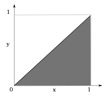
Thanks to the "uniform generator", Monte-Carlo method gives a numerical value of the integral noticed $I$. Area of integration is represented on the figure below  :


Representation of integration area

So we can distinguish two cases :

case (1) - We do 2 random sampling, one for $x$ and the other for $y$ :

\begin{equation} \textrm{Random sampling}=\left\{  
\begin{array}{lcc}  
x_{i} & \in & [0,1] \\  
y_{i} & \in & [0,1]  
\end{array}  
\right. \end{equation}

If $x_{i}>y_{i}$, then we increment $I$ in the following way : $I=I+f(x_{i},y_{i})$, else we redo a random sampling. We have done 2 random sampling and the average to lose one is 1/2.

case (2) - We do 2 random sampling like previous :

\begin{equation} \textrm{Random sampling}=\left\{  
\begin{array}{lcc}  
x_{i} &\in &[0,1] \\  
y_{i} &\in & [0,1]  
\end{array}  
\right. \end{equation}

Then, as a function of results, we increment $I$ in the following way :

\begin{equation} \textrm{Incrementation}\left\{  
\begin{array}{lcc}  
if &x_{i} > y_{i} & I=I+f(x_{i},y_{i}) \\  
if &x_{i} < y_{i} & I=I+f(y_{i},x_{i}) \\  
\end{array}  
\right. \end{equation}

The advantage here is that we use all the random sampling values unlike case (1).
Finally, one has to multiply the $I$ quantity by $(b-a)$ interval and divide by the size of random sampling $N$, so we get the numerical value of integral.

Exercise 4.2 :

A point source emits isotropically and covers an angle of $\theta _{0}$. A disk detector is positioned perpendicular to this source. So we have a cylindrical symetry with 2 angles : $\varphi $ between [0,2$\pi $] and $\theta $ as $\text {cos}(\theta _{0})<\text {cos}(\theta )<1$.

Calculate the pdf of $(\varphi ,\text {cos}\,\theta )$.

Having a generator of random values on [0,1], how will you random sample in acceptance disk a couple $(\varphi ,\text {cos}\,\theta )$ ?
With this detector, we want to do counting during equal interval time $\Delta t$. Express the distribution function for the number of recorded hits.

Correction :

Since point source emits isotropically, random variables $\varphi $ and $\text {cos}\,\theta $ follow a uniform law, respectively on [0,2$\pi $] et [$\text {cos}\,\theta _{0},1$].

We have for the $\varphi $ pdf :

\begin{equation} \text{pdf}(\varphi)=\dfrac{1}{2\pi} \end{equation}

For the $\text {cos}\,\theta $ random variable, we can write :

\begin{equation} \text{pdf}(\text{cos}\,\theta)\,d\,\text{cos}(\theta)=K\,d\,\text{cos}(\theta) \,\,\,\,\text{with $K$=constant} \end{equation}

\begin{equation} \Rightarrow  
{\large\int}_{\text{cos}\,\theta_{0}}^{1}\,\text{pdf}(\text{cos}\,\theta)\,d\,\text{cos}(\theta)=1=K\,{\large\int}_{\text{cos}\,\theta_{0}}^{1}\,d\,\text{cos}(\theta)\\  
=K\,(1-\text{cos}\,\theta_{0}) \end{equation}

\begin{equation} \Rightarrow  
K=\dfrac{1}{\,(1-\text{cos}\,\theta_{0})} \end{equation}

Given $\varphi $ and $\text {cos}\,\theta $ are independant, we conclude :

\begin{equation} \text{pdf}(\varphi,\text{cos}\,\theta)=\text{pdf}(\varphi)\,\text{pdf}(\text{cos}\,\theta)=\dfrac{1}{\,(1-\text{cos}\,\theta_{0})}\,\dfrac{1}{2\pi} \end{equation}

With a random generator between [0,1], one makes the following correspondences :

\begin{equation} \varphi=2\,\pi\,u \,\,\,\text{with}\,\,u\,\,\text{uniform on}\,\,[0,1] \end{equation}

For $\text {cos}\,\theta $, we use the relation, taking random variable $v$ as uniform on [0,1] :

\begin{equation} {\large\int}_{\text{cos}\,\theta_{0}}^{\text{cos}\,\theta}\,\dfrac{d\,\text{cos}\,\theta}{1-\text{cos}\,\theta_{0}}=\,{\large\int}_{0}^{v}\,d\,v \end{equation}

\begin{equation} \Rightarrow\text{cos}\,\theta-\text{cos}\,\theta_{0}=v(1-\text{cos}\,\theta_{0})\\  
 
\Rightarrow\text{cos}\,\theta=v+(1-v)\text{cos}\,\theta_{0} \end{equation}

The number of hits recorded during interval $\Delta t$ will follow a Poisson law.

Exercise 5.1 :

we have a set of measures $y_{i}\,\,i=1,...,n$ depending from coordinates $x_{i}$ and whose theorical model is linear $y=ax+b$. Thanks to these data, we look for determining values of $a$ and $b$.

Measures $y_{i}$ have an error $\sigma _{i}$. Firstly, coordinates $x_{i}$ are considered being without error.

- Express the $\chi ^{2}$ you have to use.
- Express the 2 equations from which you can deduce estimations for $a$ and $b$.

Correction :

With $n$ independant measures $y_{i}\,i=1,...,n$ and $n$ coordinates $x_{i}$ in a linear model $y=ax+b$, with $\sigma _{i}$ errors on $y_{i}$ and no errors on $x_{i}$, one can write the $\chi ^{2}$ as :

\begin{equation} \chi^{2}=\sum_{i=1}^{n}\,\dfrac{(y_{i}-(a\,x_{i}+b))^{2}}{\sigma_{i}^{2}} \end{equation}

One has to minimize the $\chi ^{2}$ to compute $a$ and $b$ values : one gets 2 linear equations with 2 unknowns ($a$ and $b$) :

\begin{equation} \dfrac{\partial\chi^{2}}{\partial a}=\sum_{i=1}^{n}\,\dfrac{(y_{i}-a\,x_{i}-b)\,x_{i}}{\sigma_{i}^{2}}=0 \end{equation}

and

\begin{equation} \dfrac{\partial\chi^{2}}{\partial b}=\sum_{i=1}^{n}\,\dfrac{(y_{i}-a\,x_{i}-b)}{\sigma_{i}^{2}}=0 \end{equation}

Exercise 5.2 :

Now, $x_{i}$ coordinates have $\delta _{i}$ errors.

Express the $\chi ^{2}$ which has to be used in this case.
Write the 2 equations from which you calculate $a$ and $b$ estimation. What’s the difference with previous case ?

Correction :

$\chi ^{2}$formula must be modified because we take into account of $\delta _{i}$ errors on coordinates $x_{i}$. Indeed, variance of $(y_{i}-a\,x_{i}-b)$ is not only equal to $V(y_{i})=\sigma _{i}^{2}$ :

\begin{equation} V(y_{i}-a\,x_{i}-b)=V(y_{i})+a^{2}\,V(x_{i})=\sigma_{i}^{2}+a^{2}\,\delta_{i}^{2} \end{equation}

The denominator of $\chi ^{2}$ depends on $a$ parameter :

\begin{equation} \chi^{2}=\sum_{i=1}^{n}\,\dfrac{(y_{i}-(a\,x_{i}+b))^{2}}{\sigma_{i}^{2}+a^{2}\,\delta_{i}^{2}} \end{equation}

Minimization of $\chi ^{2}$ is got by the 2 following equations :

\begin{equation} \dfrac{\partial\chi^{2}}{\partial  
a}=0\,\,\,\text{and}\,\,\,\dfrac{\partial\chi^{2}}{\partial b}=0 \end{equation}

But we notice that all these equations are not linear since the second one which minimizes the $\chi ^{2}$ with $b$ depends on powered $a$ : we have not analytical solution in this case.

Exercise 6.1 :

$\chi ^{2}$method can give estimations on parameters, $a\pm \sigma _{a}$ and $b\pm \sigma _{b}$, so a minimum value $\chi _{min}^{2}$.

We want to draw in $a,b$ plane the contour related to a given confidence level.

Express the distribution function that you use.

In this case, by fixing the confidence level, express the variation of $\chi ^{2}$ compared to $\chi _{min}^{2}$, so we could write : $\chi ^{2}(CL)=\chi _{min}^{2}+\Delta\chi_{CL}^{2}$

What value do you get with $CL=0.68$ ?

Correction :

$\chi ^{2}(CL)$term only contains second derivatives of $\chi ^{2}$ at lowest level :

\begin{equation} \dfrac{\partial^{2}\chi^{2}}{\partial  
a^{2}}\,\,\,\text{,}\,\,\dfrac{\partial^{2}\chi^{2}}{\partial  
b^{2}}\,\,\text{et}\,\,\dfrac{\partial^{2}\chi^{2}}{\partial a\partial b} \end{equation}

Concerning $\Delta \chi ^{2}$, distribution function is a $\chi ^{2}$ law with 2 freedom degrees ; pdf is written as :

\begin{equation} f(\Delta\chi^{2})=\dfrac{1}{2}\,e^{-\dfrac{\Delta\chi^{2}}{2}} \end{equation}

So for a fixed confidence level $CL$, we have :

\begin{equation} 1-CL={\large\int}_{\Delta\chi^{2}_{CL}}^{+\infty}\,\dfrac{1}{2}\,e^{-\dfrac{\Delta\chi^{2}}{2}}\,d\,\chi^{2}=e^{-\dfrac{\Delta\chi_{CL}^{2}}{2}} \end{equation}

also : $\Delta \chi ^{2}_{CL}=-2\ln(1-CL)$.

For $CL=0.68$, we have : $\Delta \chi ^{2}_{CL}=2.28$

ps : join like me the Cosmology@Home project whose aim is to refine the model that best describes our Universe

    Home | Astronomy | Sciences | Philosophy | Coding | Cv    
- dournac.org © 2003 by fab -

Back to Top