Damped Triple Pendulum Simulation with adaptative RK4

DOURNAC.ORG
	Français English

Coding > Damped Triple Pendulum Simulation with adaptative RK4 - HTML5 Canvas version

1.Introduction
2.Differential system using Euler-Lagrange
3.Lagrangian and Rayleigh's dissipation function
4.Dynamics equations of system
5.Numerical solving with Runge-Kutta 4th order
6.Simulation with HTML5 Canvas
7.Adaptative Runge-Kutta 4th order

1.Introduction :

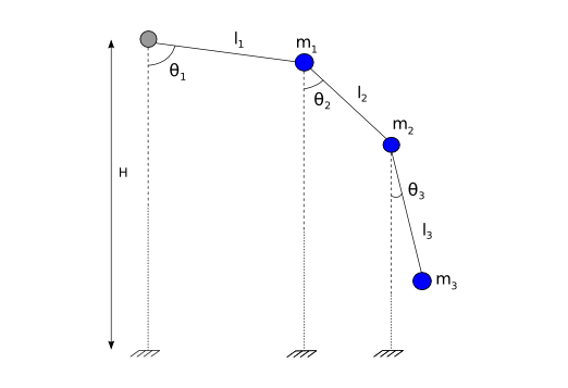
This page describes a HTML5 simulation modeling the motion of a damped triple pendulum. We get first equations of dynamics with Euler-Lagrange equations, and implement the solving of differential system with adaptative Runge-Kutta fourth-order numerical method.

2.Differential system using Euler-Lagrange :

Differential system is deduced from Euler-Lagrange equations. With $L$ the Lagrangian, $q_{i}$ each of the 3 coordinates and $\dot{q_{i}}$ their time derivatives, we can write :

\begin{equation} \dfrac{\text{d}}{\text{d}t}\bigg(\dfrac{\partial\,L}{\partial\,\dot{q_{i}}}\bigg)-\dfrac{\partial\,L}{\partial\,q_{i}}=0 \end{equation}

This equation is true when system is conservative (work of non-conservative forces is zero). When existing non-conservative forces whose work is not zero, we call them "damped" or "friction" forces. In this case, we have to add the following right member in the above equation : $\overrightarrow{F_{f}}=-\overrightarrow{\nabla_{v}}\,D_{r}$ with $D_{r}$ the Rayleigh's dissipation function. So we get :

\begin{equation} \dfrac{\text{d}}{\text{d}t}\bigg(\dfrac{\partial\,L}{\partial\,\dot{q_{i}}}\bigg)-\dfrac{\partial\,L}{\partial\,q_{i}}=-\dfrac{\partial\,D_{r}}{\partial\,\dot{q_{i}}} \end{equation}

3.Lagrangian and Rayleigh's dissipation function :

Below a graphics showing the set of variables involved in triple pendulum simulation :

**Figure 1 : Representation of a triple pendulum**

All the calculations below are done supposing that mass of each bar is negligible compared to mass of each sphere.

Lagrangian is defined by :

\begin{equation} L=\mathcal{E}_{k}-\mathcal{E}_{p} \end{equation}

with

\begin{equation} \mathcal{E}_{k}=\sum\limits_{i=1}^{3}\dfrac{1}{2}m_{i}v_{i}^{2}\,\,\,\,\,\,\,\,\, \text{et} \,\,\,\,\,\,\,\,\, \mathcal{E}_{p}=\sum\limits_{i=1}^{3}m_{i}gh_{i} \label{eq-kinetic-potential} \end{equation}

with $v_{i}^{2}=\left\Vert\dfrac{\text{d}\overrightarrow{OM_{i}}}{\text{d}t}\right\Vert^{2}=\dfrac{\text{d}\overrightarrow{OM_{i}}}{\text{d}t}\cdot\dfrac{\text{d}\overrightarrow{OM_{i}}}{\text{d}t}$ and $h_{i}$ which is related to the height of mass $i$.

Calculation of Kinetic energy - $v_{i}^{2}$ terms are equal to :

\begin{eqnarray} \left\{ \begin{aligned} v_{1}^{2}&=\dfrac{\text{d}\overrightarrow{OM_{1}}}{\text{d}t}\cdot\dfrac{\text{d}\overrightarrow{OM_{1}}}{\text{d}t}=l_{1}^{2}\dot{\theta_{1}}^{2}\\ v_{2}^{2}&=\dfrac{\text{d}\overrightarrow{OM_{2}}}{\text{d}t}\cdot\dfrac{\text{d}\overrightarrow{OM_{2}}}{\text{d}t}=\dfrac{\text{d}(\overrightarrow{OM_{1}}+\overrightarrow{M_{1}M_{2}})}{\text{d}t}\cdot\dfrac{\text{d}(\overrightarrow{OM_{1}}+\overrightarrow{M_{1}M_{2}})}{\text{d}t}\\ &=\dfrac{\text{d}\overrightarrow{OM_{1}}}{\text{d}t}\cdot\dfrac{\text{d}\overrightarrow{OM_{1}}}{\text{d}t}+\dfrac{\text{d}\overrightarrow{M_{1}M_{2}}}{\text{d}t}\cdot\dfrac{\text{d}\overrightarrow{M_{1}M_{2}}}{\text{d}t}+2\dfrac{\text{d}\overrightarrow{OM_{1}}}{\text{d}t}\cdot\dfrac{\text{d}\overrightarrow{M_{1}M_{2}}}{\text{d}t} \\ &=v_{1}^{2}+l_{2}^{2}\dot{\theta_{2}}^{2}+2 l_{1}l_{2}\dot{\theta_{1}}^{2}\dot{\theta_{2}}^{2}\cos(\theta_{1}-\theta_{2})\\ &=l_{1}^{2}\dot{\theta_{1}}^{2}+l_{2}^{2}\dot{\theta_{2}}^{2}+2 l_{1}l_{2}\dot{\theta_{1}}^{2}\dot{\theta_{2}}^{2}\cos(\theta_{1}-\theta_{2})\\ v_{3}^{2}&=\dfrac{\text{d}\overrightarrow{OM_{3}}}{\text{d}t}\cdot\dfrac{\text{d}\overrightarrow{OM_{3}}}{\text{d}t}=\dfrac{\text{d}(\overrightarrow{OM_{2}}+\overrightarrow{M_{2}M_{3}})}{\text{d}t}\cdot\dfrac{\text{d}(\overrightarrow{OM_{2}}+\overrightarrow{M_{2}M_{3}})}{\text{d}t}\\ &=\dfrac{\text{d}\overrightarrow{OM_{2}}}{\text{d}t}\cdot\dfrac{\text{d}\overrightarrow{OM_{2}}}{\text{d}t}+\dfrac{\text{d}\overrightarrow{M_{2}M_{3}}}{\text{d}t}\cdot\dfrac{\text{d}\overrightarrow{M_{2}M_{3}}}{\text{d}t} +2\dfrac{\text{d}\overrightarrow{OM_{2}}}{\text{d}t}\cdot\dfrac{\text{d}\overrightarrow{M_{2}M_{3}}}{\text{d}t}\\ &=v_{2}^{2}+l_{3}^{2}\dot{\theta_{3}}^{2}+2\dfrac{\text{d}(\overrightarrow{OM_{1}}+\overrightarrow{M_{1}M_{2}})}{\text{d}t}\cdot\dfrac{\text{d}\overrightarrow{M_{2}M_{3}}}{\text{d}t}\\ &=v_{2}^{2}+l_{3}^{2}\dot{\theta_{3}}^{2}+2 l_{1}l_{3}\dot{\theta_{1}}\dot{\theta_{3}}\cos(\theta_{1}-\theta_{3}) +2 l_{2}l_{3}\dot{\theta_{2}}\dot{\theta_{3}}\cos(\theta_{2}-\theta_{3})\\ \end{aligned} \right. \label{eq-vi2} \end{eqnarray}

Calculation of Potential energy :

The calculation is done by writting the height of each mass :

\begin{eqnarray} \begin{aligned} \mathcal{E}_{p}&=g(l_{1}+l_{2}+l_{3})(m_{1}+m_{2}+m_{3})-gl_{1}(m_{1}+m_{2}+m_{3})\cos(\theta_{1})\\ &\,\,\,\,-gl_{2}(m_{2}+m_{3})\cos(\theta_{2})-gl_{3}m_{3}\cos(\theta_{3})\\ \end{aligned} \end{eqnarray}

Calculation of dissipation function :

It is defined by :

\begin{equation} D_{r}=\dfrac{1}{2}\sum\limits_{i=1}^{3}k_{i}v_{i}^{2}\end{equation}

where $k_{i}$ corresponds to damped or friction coefficient according to $\theta_{i}$ angle and $v_{i}^{2}$ to the calculated velocities in \eqref{eq-vi2}. The right term in Euleur-Lagranage is then given by :

\begin{equation} F_{f,i}=-\dfrac{\partial D_{r}}{\partial \dot{q_{i}}} \end{equation}

4.Dynamics equations of system :

Calculating the dynamics equations can be made by hand but it may be onerous. A quicker solution is to use the Symbolic Math Toolbox. After calculating the symbolic expression of Lagrangian, we get the differential system in an automatic way. See the following Matlab source compute_diff_system.m where these operations are performed.

We describe briefly this little code :

Starting from expressions of \eqref{eq-kinetic-potential} and $v_{i}^{2}$, we get the system Lagrangian with variables $t_{i}=\theta_{i}$, $dt_{i}=\dot{\theta_{i}}$ :

% Kinetic Energy 
T=1/2*l1*l1*dt1*dt1*(m1+m2+m3)...
  +1/2*l2*l2*dt2*dt2*(m2+m3)...
  +1/2*l3*l3*dt3*dt3*m3...
  +l1*l2*dt1*dt2*cos(t1-t2)*(m2+m3)...
  +l2*l3*dt2*dt3*cos(t2-t3)*m3...
  +l1*l3*dt1*dt3*cos(t1-t3)*m3;

% Potential Energy 
V=g*(l1+l2+l3)*(m1+m2+m3)...
  -g*l1*(m1+m2+m3)*cos(t1)...
  -g*l2*(m2+m3)*cos(t2)...
  -g*l3*m3*cos(t3);

% Lagrangian 
L=T-V;

Let's take now the expression of Rayleigh's dissipation function :

% Rayleigh Dissipation function
Dr=1/2*l1*l1*dt1*dt1*(k1+k2+k3)...
   +1/2*l2*l2*dt2*dt2*(k2+k3)...
   +1/2*l3*l3*dt3*dt3*k3...
   +l1*l2*dt1*dt2*cos(t1-t2)*(k2+k3)...
   +l2*l3*dt2*dt3*cos(t2-t3)*k3...
   +l1*l3*dt1*dt3*cos(t1-t3)*k3;

% Derivative of Rayleigh function
f1=diff(Dr,dt1);
f2=diff(Dr,dt2);
f3=diff(Dr,dt3);

We have now to establish the differential system to solve. This can be done in the following way :

% Get Lagrange equations and solve for expressing theta_second
Equations=Lagrange(L,[t1,dt1,ddt1,t2,dt2,ddt2,t3,dt3,ddt3]);
[theta1_second theta2_second theta3_second]=solve(Equations(1)==-f1,...
    Equations(2)==-f2,Equations(3)==-f3,ddt1,ddt2,ddt3);

Finally, we have the 3 equations of dynamics.

Remark :

Javascript language doesn't recognize exponent character like '^'. In order to convert equations expressions from Matlab to Javascript, as 'm1^2', to 'm1*m1', we can use the terminal command below (with sed) :

sed -i 's/\([^(*+\/^-]*\(([^)]*)\)\?\)\^2/\1\*\1/g' diff_system.txt

We decided not to use the 'Math.pow' function since it is disadvantageous from an optimization point of view with integer power exponent.

5.Numerical solving with Runge-Kutta 4th order :

This numerical method is appropriate to the following kind of problems :

\begin{equation} \dfrac{\text{d}y}{\text{d}t}=\Psi(t,y) \label{eq-rk4-basic} \end{equation}

with known initial conditions $t_{0}$ and $y_{0}$. Then, recurrence formula is :

\begin{equation} y_{i+1}=y_{i}+\dfrac{(k_{1}+2k_{2}+2k_{3}+k_{4})}{6} \end{equation} with \begin{equation} k_{1}=h\Psi(t_{i},y_{i})\,\,\,\,\,\,\,\,\,\,\,\,\,\,\,\,\,\,k_{2}=h\Psi(t_{i}+\dfrac{h}{2},y_{i}+\dfrac{k_{1}}{2})\\ k_{3}=h\Psi(t_{i}+\dfrac{h}{2},y_{i}+\dfrac{k_{2}}{2})\,\,\,\,\,\,\,\,\,\,\,\,\,\,\,\,\,\,k_{4}=h\Psi(t_{i}+h,y_{i}+k_{3})\\ \end{equation}

For a system of equations involving the second derivatives, we use a vectorial approach. In our case, we set the differential system to this form :

\begin{eqnarray} \left\{ \begin{aligned} x"&=F(x,x',y,y',z,z')\\ y"&=G(x,x',y,y',z,z')\\ z"&=H(x,x',y,y',z,z') \end{aligned} \right. \label{eq-diff-rk4} \end{eqnarray}

Taking $u=\dfrac{\text{d}x}{\text{d}t}$, $v=\dfrac{\text{d}y}{\text{d}t}$, $w=\dfrac{\text{d}z}{\text{d}t}$, and defining the vector $\overrightarrow{V}$ :

\begin{equation} \overrightarrow{V}=\begin{bmatrix} x \\ u \\ y \\ v \\ z \\ w\end{bmatrix} \end{equation}

We can reformulate the differential system to an equivalent form of \eqref{eq-rk4-basic} :

\begin{equation} \dfrac{\text{d}\overrightarrow{V}}{\text{d}t}=\overrightarrow{U}(\overrightarrow{V})=\begin{bmatrix} u(x,x',y,y',z,z') \\ F(x,x',y,y',z,z') \\ v(x,x',y,y',z,z') \\ G(x,x',y,y',z,z') \\ w(x,x',y,y',z,z') \\ H(x,x',y,y',z,z')\end{bmatrix} \end{equation}

Runge-Kutta coeffcients are calculated this way :

\begin{equation} \overrightarrow{k_{1}}=h\overrightarrow{U}(\overrightarrow{V_{n}})\,\,\,\,\,\,\,\,\,\,\,\,\,\,\,\,\,\,\overrightarrow{k_{2}}=h\overrightarrow{U}(\overrightarrow{V_{n}}+\dfrac{\overrightarrow{k_{1}}}{2})\\ \overrightarrow{k_{3}}=h\overrightarrow{U}(\overrightarrow{V_{n}}+\dfrac{\overrightarrow{k_{2}}}{2})\,\,\,\,\,\,\,\,\,\,\,\,\,\,\,\,\,\,\overrightarrow{k_{4}}=h\overrightarrow{U}(\overrightarrow{V_{n}}+\overrightarrow{k_{3}})\\ \end{equation}

and recurrence formula is written :

\begin{equation} \overrightarrow{V_{n+1}}=\overrightarrow{V_{n}}+\dfrac{\overrightarrow{k_{1}}+2\overrightarrow{k_{2}}+2\overrightarrow{k_{3}}+\overrightarrow{k_{4}}}{6} \end{equation}

6.Simulation with HTML5 Canvas :

Below this canvas can simulate the motion of a triple pendulum. The total length of axis is fixed to 3 meters, each initial mass is set to 1 kg and its starting rotation speed is set to $5\,\text{rad.s}^{-1}$. You can drag'n drop with mouse each mass in order to set wanted initial position.

Axis lengths
$\mathbf{M_{1}}$	$\mathbf{M_{2}}$	$\mathbf{M_{3}}$
$\mathbf{\Theta_{1}}$	$\mathbf{\Theta_{2}}$	$\mathbf{\Theta_{3}}$
$\mathbf{\dot{\Theta}_{1}}$	$\mathbf{\dot{\Theta}_{2}}$	$\mathbf{\dot{\Theta}_{3}}$
$\mathbf{K_{1}}$	$\mathbf{K_{2}}$	$\mathbf{K_{3}}$

The Canvas HTML5 source is available on this link triple_pendulum.js. We begin by initializing graphics interface and then define functions corresponding to the differential system. Afterwards, adaptative Runge-Kutta 4th is implemented to compute next positions and velocities. Once getting these variables, we update the graphics display of triple pendulum.

7.Adaptative Runge-Kutta 4th order :

Under some choices of axes length, or a relative important difference between the 3 masses of pendulum, angles $\theta_{i}$ may to vary very quickly. In these cases, a smaller time step than the default one ($h=0.005$) has to be used for avoiding divergence. This method is called "Adaptative Runke-Kutta". Indeed, the goal is to get a time step which is adapted as a function of the variability of computed variables : timestep is decreased when they are changing roughly and increased when variation is slowly.

For estimating this variability, we set a minimal tolerance beyond which one must reduce the time step. This is done by comparing the variables got by one iteration wih $h$ current time step and ones got by two iterations with current $h/2$. If difference is greater than tolerance, we set a smaller step, otherwise we increase it.

Here is a description of this algorithm :

1 function ProcessNext() {
2
3    // Correction for current step
4    var factor_correction;
5
6    // Compute RK4 coefficients
7    k[0][0]=h*dt1;
8    k[0][1]=h*F1(t1, dt1, t2, dt2, t3, dt3, g, l1, l2, l3, ...
9    ...
10    ...
11    k[3][4]=h*(dt3+k[2][5]);
12    k[3][5]=h*F3(t1+k[2][0], dt1+k[2][1], t2+k[2][2], ...
13
14    // Save first computed variables
15    t1_1=t1;
16    dt1_1=dt1;
17    ...
18    ...
19    t3_1=t3;
20    dt3_1=dt3;
21
22    t1_2=t1;
23    dt1_2=dt1;
24    ...
25    ...
26    t3_2=t3;
27    dt3_2=dt3;
28
29    // Compute Next positions
30    t1=t1+(k[0][0]+2*k[1][0]+2*k[2][0]+k[3][0])/6;
31    dt1=dt1+(k[0][1]+2*k[1][1]+2*k[2][1]+k[3][1])/6;
32    ...
33    ...
34    t3=t3+(k[0][4]+2*k[1][4]+2*k[2][4]+k[3][4])/6;
35    dt3=dt3+(k[0][5]+2*k[1][5]+2*k[2][5]+k[3][5])/6;
36
37    // 2 Loops for RK4 with h/2
38    for (i=0; i<2; i++) {
39       // Compute RK4 coefficients with h/2
40       k[0][0]=h/2*dt1_1;
41       k[0][1]=h/2*F1(t1_1, dt1_1, t2_1, dt2_1, t3_1, dt3_1, g,  ...
42       ...
43       ...
44       k[3][4]=h/2*(dt3_1+k[2][5]);
45       k[3][5]=h/2*F3(t1_1+k[2][0], dt1_1+k[2][1], t2_1+k[2][2], ...
46
47       // Compute Next positions
48       t1_1=t1_1+(k[0][0]+2*k[1][0]+2*k[2][0]+k[3][0])/6;
49       dt1_1=dt1_1+(k[0][1]+2*k[1][1]+2*k[2][1]+k[3][1])/6;
50       ...
51       ...
52       t3_1=t3_1+(k[0][4]+2*k[1][4]+2*k[2][4]+k[3][4])/6;
53       dt3_1=dt3_1+(k[0][5]+2*k[1][5]+2*k[2][5]+k[3][5])/6;
54    }
55
56    // Comparison with h and h/2 results
57    max_delta = Math.max(Math.abs(t1-t1_1),Math.abs(t2-t2_1),Math.abs(t3-t3_1));
58
59    // Factor correction
60    factor_correction=Math.pow(Err/max_delta,0.2);
61
62    // Set new step
63    h=h*factor_correction;
64
65    if (max_delta >= Err) {
66      // Restore initial values
67      t1=t1_2;
68      dt1=dt1_2;
69      ...
70      ...
71      t3=t3_2;
72      dt3=dt3_2;
73      // Recompute with a smaller step (factor_correction < 1)
74      ProcessNext();
75    }
76    else {
77      // Draw Canvas - max_delta less than error (factor_correction > 1)
78      DrawPend(canvas);
79    }
80 }

ps : join like me the Cosmology@Home project whose aim is to refine the model that best describes our Universe