MPI Numerical solving of the 2D Heat equation

DOURNAC.ORG
	Français English

Coding > MPI Parallelization for numerically solving the 2D Heat equation

1.Execution
2.Unsteady Heat equation 2D
3.Discretization : FTCS scheme

3.1 Spatial discretization
3.2 Temporal discretization

4.Convergence criterion
5.MPI Implementation

5.1 Cartesian topology of processes
5.2 Remarks on contiguity
5.3 Communications between processes

6.Results
7.Benchmark

1.Execution :

Sequential and parallelized codes are in the following archives :

C language version : Heat2D_MPI_Solving_C.tar.gz

Fortran 90 version : Heat2D_MPI_Solving_F90.tar.gz

Make sure at the execution of parallel code (with "mpirun" command) that number of processes equals to product of subdomains number along x by subdomains number along y ( "x_domains" and "y_domains" parameters in "param" input file ) :

$ cat param
  size_x
1024
  size_y
1024
  x_domains
16
  y_domains
16
  MaxStep
100000000
  dt
1.0e-1
  cnv_tol
1.0e-1

We take in this case 256 processes, then running command is :

$ mpirun -np 256 ./explicitPar

  Time step too large in 'param' file - Taking convergence criterion

  Time step = 2.374899779E-07

  Convergence = 0.100000000 after 40595 steps

  Problem size = 1048576

  Wall Clock = 487.038250208

  Computed solution in outputPar.dat file

2.Unsteady Heat equation 2D :

The general form of Heat equation is :

\begin{equation} \dfrac{\partial T}{\partial t}=\kappa\,\Delta T\,\,\,\,\,\,\text{with}\,\,\,\,\,\Delta=\sum_{i=1}^{n}\dfrac{\partial^{2}}{\partial x_{i}^{2}}\,\,\,\,\text{the Laplacian in $n$ dimension} \label{eq1} \end{equation}

$\kappa$ coefficient is the thermal conductivity. So, 2D Heat equation can be written :

\begin{equation} \dfrac{\partial\theta}{\partial t}=\kappa\,\bigg(\dfrac{\partial^{2}\theta}{\partial x^{2}}+\dfrac{\partial^{2}\theta}{\partial y^{2}}\bigg) \label{eq2} \end{equation}

3.Discretization : FTCS scheme

We use the FTCS (Forward-Time Central-Space) method which is part of Finite Difference Methdod and commonly used to solve numerically heat diffusion equation and more generally parabolic partial differential equations. This scheme is based on central difference in space and the forward Euler method in time. So discretization has 2 types : spatial and temporal. To use light notations, we write the 2D spatial discretized element $(i,j)$ at time $n$ under the form $\theta_{\,i\,,\,j}^{\,n}$.

3.1 Spatial discretization :

We start by discretize into 1D case the right member, i.e in spatial domain. For this, we use the two following Taylor series :

\begin{equation} \theta_{m+1}=\theta(x_{m}+h)=\theta(x_{m})+h\,\theta'(x_{m})+\dfrac{h^{2}}{2}\,\theta''(x_{m})+\dfrac{h^{3}}{6}\,\theta^{'''}(x_{m})+O(h^{4}) \label{eq3} \end{equation} \begin{equation} \theta_{m-1}=\theta(x_{m}-h)=\theta(x_{m})-h\,\theta'(x_{m})+\dfrac{h^{2}}{2}\,\theta''(x_{m})-\dfrac{h^{3}}{6}\,\theta^{'''}(x_{m})+O(h^{4}) \label{eq4} \end{equation}

By adding the relations \eqref{eq3} and \eqref{eq4}, we get an expression of second derivate at $x_{m}$ point :

\begin{equation} \theta''(x_{m})=\dfrac{\theta_{m+1}-2\theta_{m}+\theta_{m-1}}{h^{2}}+O(h^{2}) \label{eq5} \end{equation}

In 2D case, we get the same relations for $y$ variable. By taking $h_{x}=size_{x}/N_{x}$ , $h_{y}=size_{y}/N_{y}$ and with convention $\theta(x_{i},y_{j})=\theta_{\,i\,,j}$, we have :

\begin{equation} \dfrac{\partial^{2}\theta}{\partial x^{2}}+\dfrac{\partial^{2}\theta}{\partial y^{2}}=\dfrac{\theta_{\,i+1\,,\,j}-2\theta_{\,i\,,\,j}+\theta_{\,i-1\,,\,j}}{h_{x}^{2}}+\dfrac{\theta_{\,i\,,\,j+1}-2\theta_{\,i\,,\,j}+\theta_{\,i\,,\,j-1}}{h_{y}^{2}} \label{eq6} \end{equation}

3.2 Temporal discretization :

Left member of equation \eqref{eq2} can be expressed :

\begin{equation} \dfrac{\partial \theta_{\,i\,,\,j}^{\,n}}{\partial t}=\dfrac{\theta_{\,i\,,\,j}^{\,n+1}-\theta_{\,i\,,\,j}^{\,n}}{\Delta t} \label{eq7} \end{equation}

Thus, by combining equations \eqref{eq2} and \eqref{eq6}, recurrence formula equals to :

\begin{equation} \theta_{\,i\,,\,j}^{\,n+1}=\theta_{\,i\,,\,j}^{\,n}+\kappa \Delta t\,\bigg[\dfrac{\theta_{\,i+1\,,\,j}^{\,n}-2\theta_{\,i\,,\,j}^{\,n}+ \theta_{\,i-1\,,\,j}^{\,n}}{h_{x}^{2}}+\dfrac{\theta_{\,i\,,\,j+1}^{\,n}-2\theta_{\,i\,,\,j}^{\,n}+\theta_{\,i\,,\,j-1}^{\,n}}{h_{y}^{2}}\bigg] \label{eq8} \end{equation}

This formula is implemented in this way for the C language parallel version (cf explUtilPar.c file) ; You can notice that xs, xe, ys, ye (with "s" for "start" and "e" for "end") variables represent the coordinates of the subdomain corresponding to the current process of rank "me" :

   // Factors for explicit scheme
   diagx = -2.0 + hx*hx/(2*k0*dt);
   diagy = -2.0 + hy*hy/(2*k0*dt);
   weightx = k0 * dt/(hx*hx);
   weighty = k0 * dt/(hy*hy);

   // Perform an explicit update on the points within the domain
   for (i=xs[me];i<=xe[me];i++)
     for (j=ys[me];j<=ye[me];j++)
       x[i][j] = weightx*(x0[i-1][j] + x0[i+1][j] + x0[i][j]*diagx)
               + weighty*(x0[i][j-1] + x0[i][j+1] + x0[i][j]*diagy)

4.Convergence criterion :

Convergence criterion links the exact solution with the numerically computed solution. If we have $h_{x}=h_{y}=h$, explicit schema \eqref{eq8} is steady if :

\begin{equation} \Delta t\leqslant \dfrac{h^{2}}{4\kappa} \label{eq9} \end{equation}

Given a spatial discretizion step, this stability condition gives an estimation for choosing the time step $\Delta t$ :

\begin{equation} \Delta t=\dfrac{1}{4\kappa}\,\text{min}(h_{x},h_{y})^{2} \label{eq10} \end{equation}

5.MPI Implementation :

We discuss in this part about the way that numerical solving is structured and implemented using "Message Passing Interface" (MPI) API.

5.1 Cartesian topology of processes :

We are going to breakdown domain (also named grid) into subdomains assigning for each one a process. Gain on runtime is achieved since computing iterative schema is done parallely and updates for the 4 sides of a given subdomain is performed with communications of surrounding processes : we called this breakdown a "Cartesian topology of processes" because subdomains are squared or rectangular. Convention taken here, for indices of 2D arrays with both Fortran90 and C languages, is (i,j)=(row,column). Below an example showing the breakdown with 8 processes along x_domains=2 and y_domains=4 :

Figure 1 : Ranks of processes with convention (row,column)$\,\equiv\,$(x_domains,y_domains)

To create this topology, we use the MPI_Cart_create function. Caution, convention imposed by MPI for this function is the opposite of our convention for 2D arrays, i.e (i,j)=(row,column)$\,\equiv\,$(y_domains,x_domains) turns into (row,column)$\,\equiv\,$(x_domains,y_domains) as it is illustrated in figure above. So one has to switch (Ox) and (Oy) axis in the following way :

C language :

// Invert (Ox,Oy) classic convention
dims[0] = y_domains;
dims[1] = x_domains;
MPI_Cart_create(comm, ndims, dims, periods, reorganisation, &comm2d);

Fortran90 :

! Invert (Ox,Oy) classic convention
dims(1) = y_domains
dims(2) = x_domains
call MPI_Cart_create(MPI_COMM_WORLD, ndims, dims, periods, reorganisation, comm2d, infompi)

5.2 Remarks on contiguity :

With Fortran, elements of 2D array are memory aligned along columns : it is called "column major". In C language, elements are memory aligned along rows : it is qualified of "row major".

As we will see below into part 5.3, one has to exchange rows and columns between processes. C language naturally allows to handle data with row type and Fortran90 with column type. To get both functionalities for each language, we define, into function updateBound, "column" type (column_type) and "row" type (row_type) respectively for C language and Fortran90.

C language :

// Create column data type to communicate with East and West neighBors
MPI_Type_vector(xcell, 1, size_total_y, MPI_DOUBLE, &column_type);
MPI_Type_commit(&column_type);

Fortran90 :

! Create row data type to communicate with South and North neighBors
call MPI_Type_vector(ycell, 1, size_tot_x, MPI_DOUBLE_PRECISION, row_type, infompi)
call MPI_Type_commit(row_type, infompi)

From an optimization point of view, we have to make sure to iterate in loops on right indices : the most inner loop must be executed on the first index for Fortran90 and on the second one for C language.

5.3 Communications between processes :

Parallelization implies to use communications between the processes of each subdomain. As we can see in the code snippet below, for a given iteration process with rank "me", we compute the next values to the corresponding subdomain with "computeNext" function, then we send with "updateBound" rows and columns respectively to processes located in North-South and East-West of the current process "me".

   // Main loop : until convergence
   while (!convergence) {
     // Increment step and time
     step = step+1;
     t = t+dt;
     // Perform one step of the explicit scheme
     computeNext(x0, x, dt, hx, hy, &localDiff, me, xs, ys, xe, ye, k0);
     // Update the partial solution along the interface
     updateBound(x0, neighBor, comm2d, column_type, me, xs, ys, xe, ye, ycell);
     // Sum reduction to get global difference
     MPI_Allreduce(&localDiff, &result, 1, MPI_DOUBLE, MPI_SUM, comm);
     // Current global difference with convergence
     result= sqrt(result);
     // Break if convergence reached or step greater than maxStep
     if ((result<epsilon) || (step>maxStep)) break;
   }

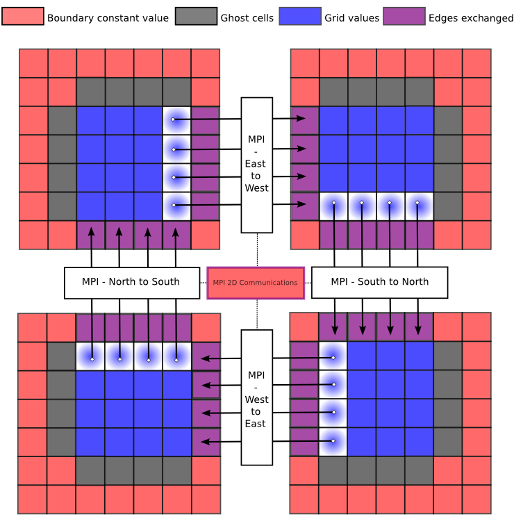
The following figure shows an example of communication for a breaking down of global domain into 4 subdomains, which means with 4 processes :

**Figure 2 : Example of communications between 4 processes**

Note that ghost cells are initialized at the beginning of code to the constant value of the edge of grid.

Below the content of "updateBound" function which defines the communications between processes :

C language :

// North/South communication
// Send boundary to North and receive from South
MPI_Sendrecv(&x[xe[me]][ys[me]], ycell, MPI_DOUBLE, neighBor[N], flag,
             &x[xs[me]-1][ys[me]], ycell, MPI_DOUBLE, neighBor[S], flag,
             comm2d, &status);
// Send boundary to South and receive from North
MPI_Sendrecv(&x[xs[me]][ys[me]], ycell, MPI_DOUBLE, neighBor[S], flag,
             &x[xe[me]+1][ys[me]], ycell, MPI_DOUBLE, neighBor[N], flag,
             comm2d, &status);

// East/West communication
// Send boundary to East and receive from West
MPI_Sendrecv(&x[xs[me]][ye[me]], 1, column_type, neighBor[E], flag,
             &x[xs[me]][ys[me]-1], 1, column_type, neighBor[W], flag,
             comm2d, &status);
// Send boundary to West and receive from East
MPI_Sendrecv(&x[xs[me]][ys[me]], 1, column_type, neighBor[W], flag,
             &x[xs[me]][ye[me]+1], 1, column_type, neighBor[E], flag,
             comm2d, &status);

Fortran90 :

! North/South communication
! Send boundary to North and receive from South
call MPI_Sendrecv(x(xe(me), ys(me)), 1, row_type, neighBor(N), flag, &
                  x(xs(me)-1, ys(me)), 1, row_type, neighBor(S), flag, &
                  comm2d, status, infompi)
! Send boundary to South and receive from North
call MPI_Sendrecv(x(xs(me), ys(me)), 1, row_type, neighBor(S), flag, &
                  x(xe(me)+1, ys(me)), 1, row_type, neighBor(N), flag, &
                  comm2d, status, infompi)

! East/West communication 
! Send boundary to East and receive from West
call MPI_Sendrecv(x(xs(me), ye(me)), xcell, MPI_DOUBLE_PRECISION, neighBor(E), flag, &
                  x(xs(me), ys(me)-1), xcell, MPI_DOUBLE_PRECISION, neighBor(W), flag, &
                  comm2d, status, infompi)
! Send boundary to West and receive from East
call MPI_Sendrecv(x(xs(me), ys(me)), xcell, MPI_DOUBLE_PRECISION, neighBor(W), flag, &
                  x(xs(me), ye(me)+1), xcell, MPI_DOUBLE_PRECISION, neighBor(E), flag, &
                  comm2d, status, infompi)

6.Results :

To get an animated gif showing the temporal evolution of diffusion, we need output data files at different time intervals. We use this script generate_outputs_heat2d which will generate it. Then, we use the Matlab script generate_gif_heat2d.m to generate a gif file. Here is an animation made with a 256x96 mesh :

**Figure 3 : Animated Gif showing temperature evolution on domain**

7.Benchmark :

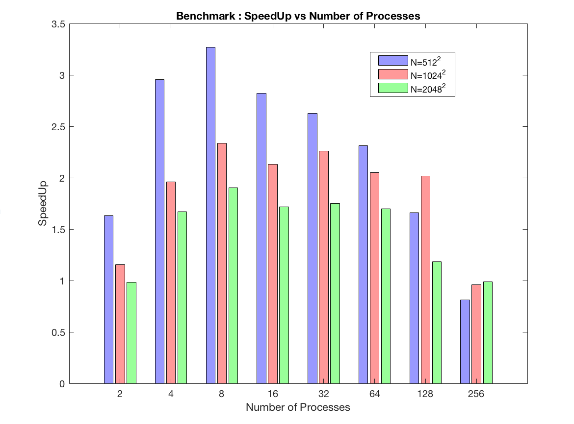
To evaluate the performance of the code, we do a benchmark by varying the number of processes for three different grid sizes (512^2, 1024^2, 2048^2). The script run_benchmark_heat2d allows to get execution time for each of these two parameters.

The following graph, produced with the Matlab script plot_benchmark_heat2d.m , synthesizes this benchmark :

**Figure 4 : SpeedUp as a function of processes number and size of domain**

Performance for one single process represents the execution of the sequential code. Except for N = 2048, the runtimes for a number of processes from 2 to 128 are lower than the sequential version. We can see that the best performance is done with 8 processes, regardless of the size of the mesh. This could be explained by the fact that this benchmark has been achieved with 8-core i7 processor. Indeed, Core i7 implements "Hyper-Threading" : this multitasking technique allows a physical optimization for 8 processes and a logical optimization for a higher number of processes. For a number of processes equal to 256, we find roughly the same time as with sequential code; this reflects the overhead caused by the high number of communications on the effective computation time in each subdomain of the grid.

ps : join like me the Cosmology@Home project whose aim is to refine the model that best describes our Universe